Pan-European Maps - Introduction

Background

Pesticides are used and released into the European environment. Despite their use being regulated by stringent pre-market evaluation, in the environment, they create mixtures of multiple substances with the potential to negatively affect soil and aquatic organisms. While the monitoring data are limited, tools may be developed to estimate pesticide emissions and their distribution in the environment and accumulated levels based on existing data on pesticide use and properties.

How it works

We provide detailed spatial maps that estimate where pesticides are most likely to accumulate in Europe’s environment, including in soils, rivers and lakes, and the air. These maps cover 121 pesticides and were developed by combining real-world data on how and where pesticides are used with models that simulate the movement of pesticides through nature and the environment.

What it offers

• These maps help in understanding where pesticides end up in the environment, even in areas far from where they were applied.
• They highlight places where nature or people may be more exposed to pesticide pollution.
• This information can help governments and researchers make better decisions to protect public health and the environment from exposure to agricultural pesticides.

The goal is to support smarter, more sustainable farming and help reduce the harmful impacts of pesticide use across Europe.

Limitations

The tool must be used carefully, knowing all its limitations - see "Interpretation guide" below.

Background

Pesticide mixtures occur in soil and water. Despite the regulation, limited monitoring data document that. However, monitoring can hardly cover the large European area; therefore, modelling and estimation are the approaches available to provide pan-European maps of pesticide environmental concentrations. To fulfill the EU’s goals under the Green Deal and Farm to Fork Strategy, policy-makers and regulators need a pan-European perspective on potential environmental exposure to pesticides to prioritize pesticide-reduction strategies.

How it works

The SPRINT Toolbox includes geospatial maps showing estimated environmental concentrations of pesticide active ingredients across the EU from their use across different agricultural crops. Separate maps are provided for agricultural soil, natural soil, freshwater bodies, and the atmosphere as the main environmental compartments. The maps result from combining pesticide usage data (years 2016 to 2020), environmental emission modeling, and geospatial fate and transport modeling. The work aligns with the EU’s goals under the Green Deal and Farm to Fork Strategy by improving transparency and supporting science-based pesticide management and impact reduction.

What it offers

The geospatial pesticide concentration maps can support:

• Targeted policy interventions in high-risk areas for pesticide accumulation and exposure.
• Risk prioritization for improving environmental quality and reducing potential human health impacts from pesticide emissions.
• Monitoring and evaluation of pesticide regulation effectiveness, such as pesticide reduction efforts.
• Strategic planning for reducing pesticide use or exposure in line with sustainable agricultural and public health goals.

By identifying vulnerable compartments and geographic hotspots, these maps allow policymakers to prioritize resources and set regulatory focus where the need for risk mitigation is greatest. 

Limitations

The tool must be used carefully knowing all its limitations - see "Interpretation guide" below.

The chemical concentration maps in different environmental media (agricultural soil, natural soil, freshwater, and air) in this tool have been created for selected substances by combining a global pesticide usage dataset, an emission distribution model, and the geospatial Pangea model, to indicate the environmental fate of pesticides, which influences impacts on ecosystems and human health. The details of steps taken for the projection of pesticide active ingredient concentrations in different compartments can be found in the following:

Global pesticide usage data: Pesticide usage data have been obtained for the years 2016-2020 from an external data provider (https://lexagri.com/products/agrowin). These data have a high granularity, providing actual pesticide use information at the level of crop, country, active ingredient, crop growth stage, and application method. The data were projected on globally spatialized crop production maps at a 5×5 arcminute resolution using the Spatial Production Allocation Model (https://mapspam.info).

Pesticide emissions (primary distribution) to different compartments: The emission distribution model PestLCI used information on crop, crop growth stage and pesticide application method to derive a set of environmental primary emission distributions, building on a mass balance after pesticide application (Dijkman et al., 2012; Nemecek et al., 2022; Zhang et al., 2024). Emission compartments include air, field crop surface, field soil surface, and off-field surface areas that include other agricultural fields, natural soil surfaces and freshwater surfaces. Environmental processes beyond primary distribution among above-mentioned compartments are considered in subsequent fate models. For breaking off-field area into the defined compartments, spatialized land use data were extracted from 2018 version of the Copernicus European Landcover (Büttner et al., 2004).

Geospatial Pangea model: This model builds a set of grids for relevant compartments using its GIS engine and a set of Environmental Models (EMs), which simulate physical systems such as the atmosphere, hydrology, and terrestrial environments. This system is called geometric system, and all geo-referenced data are projected in this system. This system includes grid cells with homogenous (e.g., air) and inhomogeneous (e.g., soil) compartments. The geometric system includes following grids:

• A 3D atmospheric grid of 17 layers covering altitudes ranging from around 100 m to 15 km. This is based on the default GEOS-Chem layers which is the wind field dataset (Bey et al., 2001). This dataset is developed with a time resolution of 6 hours and spatial resolution of 2° x 2.5°, provides wind velocities for each defined atmospheric layer in different directions. This dataset is then interpolated to the resolution for the geometry of the atmospheric grid.
• A terrestrial grid of clusters delineated by watersheds delivering to a global ocean, which is based on the catchment-based HydroBASINS dataset (https://www.hydrosheds.org), which provides separate river and lake datasets. This dataset has been used as a basis for computing flows between watersheds.

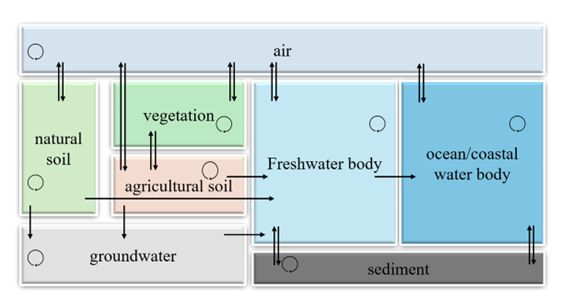
 The gridded data and geometric and topological parameters are re-indexed into a virtual system to split inhomogeneous contents into homogenous cells. With homogenous cells, pesticide mass evolution in compartments can be described using first-order differential equations with constant coefficients. Using these re-indexed parameters and a set of Environmental Processes Models (EPMs), Pangea builds a mathematical compartmental system, which is solved for environmental concentrations of pesticides at steady state. The solution is re-indexed backward to the relevant grids for analysis and visualization. EPMs are specific to each compartment for the elimination process (degradation, and advection), to each pair of compartments for transfer processes (diffusion, deposition, and runoff) and to each exposure pathway for exposure processes. EPMs are based on IMPACT 2002 (Margni et al., 2004; Pennington et al., 2005), and USEtox (Rosenbaum et al., 2008). The following figure (Fig. 1) shows considered compartments, fate and environmental processes in Pangea (Wannaz et al., 2018):

Fig. 1. Set of compartments and related environmental processes involved in Pangea

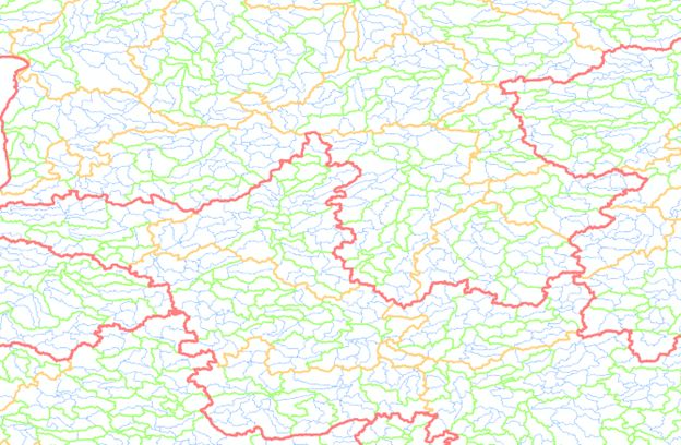
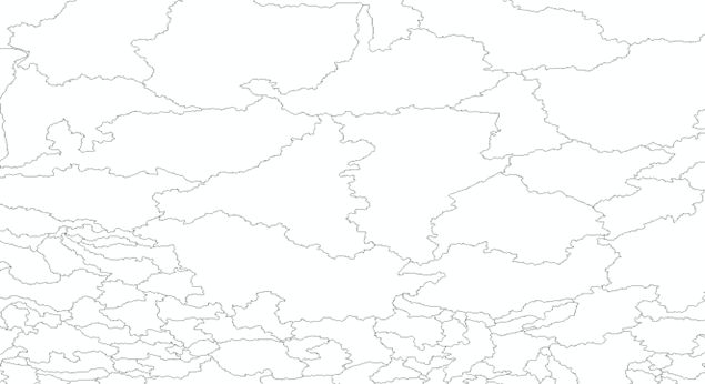
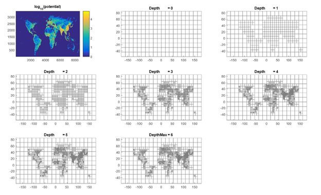
Defining resolution for projecting the results: For specifying constraints on the output map resolution, Pangea uses a practical solution as a basis for building multi-scale grids, called refinement potential (RP). It is by definition a global scalar field whose value in each point of the globe defines the user "interest for high resolution". In practice, it is a raster that results from multiple, weighted contributions. In the SPRINT project, the refinement potential was defined based on the weight of terrestrial catchment areas based on the ratio of the population to freshwater volume and ecotoxicity impacts of pesticides related to the emissions sources and regions, so that the areas with higher population/volume ratio and higher potential ecotoxicity impacts from pesticide use get higher resolution. Figures 2 and 3 show the scales used for this process and also refined maps.

(a)    Terrestrial grids used for refinement potential process

(b)   Refined terrestrial grids

Fig. 2. (a) Different levels of terrestrial grids used for refining the grids based on HydroBASINS dataset. Watershed levels 4 (red line), 6 (orange line), 8 (green line), and 10 (blue line). Higher levels represent higher resolution (First picture). And (b) shows the refined grids based on defined constraints

Fig. 3. Overview of refinement procedure for atmospheric grids. Further depths show higher resolution based on user-defined constraints

References:

• Bey, I., Jacob, D.J., Yantosca, R.M., Logan, J.A., Field, B.D., Fiore, A.M., Li, Q., Liu, H.Y., Mickley, L.J., Schultz, M.G., 2001. Global modeling of tropospheric chemistry with assimilated meteorology: Model description and evaluation. J. Geophys. Res. Atmos. 106, 23073–23095. https://doi.org/10.1029/2001JD000807
• Büttner, G., Feranec, J., Jaffrain, G., Mari, L., Maucha, G., Soukup, T., 2004. THE CORINE LAND COVER 2000 PROJECT. EARSeL eProceedings 3, 331–346.
• Dijkman, T.J., Birkved, M., Hauschild, M.Z., 2012. PestLCI 2.0: A second generation model for estimating emissions of pesticides from arable land in LCA. Int. J. Life Cycle Assess. 17, 973–986. https://doi.org/10.1007/s11367-012-0439-2
• Margni, M., Pennington, D.W., Amman, C., Jolliet, O., 2004. Evaluating multimedia/multipathway model intake fraction estimates using POP emission and monitoring data. Environ. Pollut. 128, 263–277. https://doi.org/10.1016/J.ENVPOL.2003.08.036
• Nemecek, T., Antón, A., Basset-Mens, C., Gentil-Sergent, C., Renaud-Gentié, C., Melero, C., Naviaux, P., Peña, N., Roux, P., Fantke, P., 2022. Operationalising emission and toxicity modelling of pesticides in LCA: the OLCA-Pest project contribution. Int. J. Life Cycle Assess. 27, 527–542. https://doi.org/10.1007/s11367-022-02048-7
• Pennington, D.W., Margni, M., Ammann, C., Jolliet, O., 2005. Multimedia fate and human intake modeling: Spatial versus nonspatial insights for chemical emissions in Western Europe. Environ. Sci. Technol. 39, 1119–1128. https://doi.org/10.1021/ES034598X/SUPPL_FILE/ES034598XSI20041228_113315.PDF
• Rosenbaum, R.K., Bachmann, T.M., Gold, L.S., Huijbregts, M.A.J., Jolliet, O., Juraske, R., Koehler, A., Larsen, H.F., MacLeod, M., Margni, M., McKone, T.E., Payet, J., Schuhmacher, M., Van De Meent, D., Hauschild, M.Z., 2008. USEtox - The UNEP-SETAC toxicity model: Recommended characterisation factors for human toxicity and freshwater ecotoxicity in life cycle impact assessment. Int. J. Life Cycle Assess. 13, 532–546. https://doi.org/10.1007/S11367-008-0038-4
• Wannaz, C., Fantke, P., Jolliet, O., 2018. Multiscale Spatial Modeling of Human Exposure from Local Sources to Global Intake. Environ. Sci. Technol. 52, 701–711. https://doi.org/10.1021/acs.est.7b05099
• Zhang, Y., Li, Z., Reichenberger, S., Gentil-Sergent, C., Fantke, P., 2024. Quantifying pesticide emissions for drift deposition in comparative risk and impact assessment. Environ. Pollut. 342, 123135. https://doi.org/10.1016/J.ENVPOL.2023.123135